How Databases Actually Store Data: B-Trees vs LSM-Trees

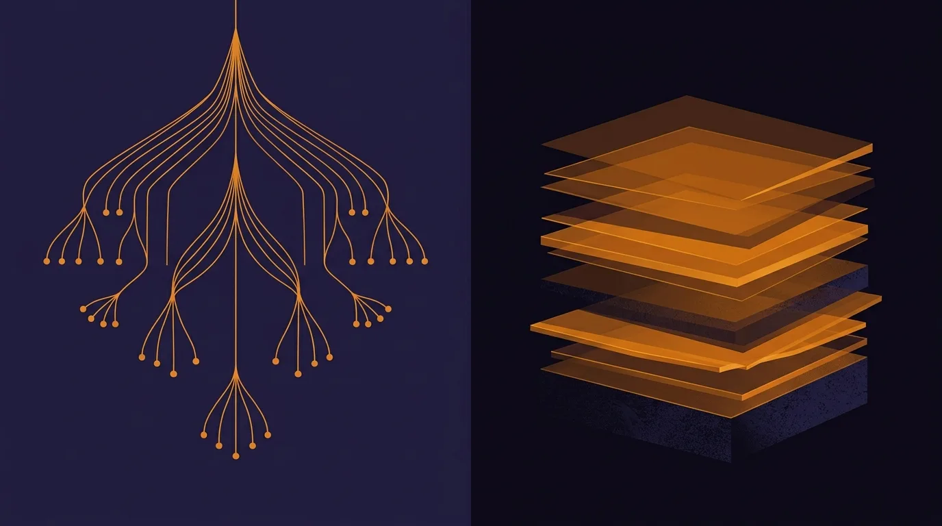
Every database promises the same interface: put a key in, get a key back, scan a range. Underneath that interface, two storage engine designs dominate almost everything you will touch in production, and they make opposite bets about what is expensive.

PostgreSQL, MySQL’s InnoDB, and SQLite build on B-trees. RocksDB, LevelDB, and Cassandra build on log-structured merge trees (LSM-trees). Both are decades-old ideas, both are still the default choice for new systems, and the difference between them explains a surprising amount of database behavior you have probably seen without knowing why: why write-heavy time-series workloads reach for Cassandra, why Postgres index bloat is a recurring maintenance chore, and why RocksDB-backed stores periodically spike CPU on “compaction.”

B-trees: optimize for reads, pay on write

A B-tree is a balanced, multi-way tree of fixed-size pages. PostgreSQL’s implementation is a representative example: the tree has a fixed metapage, internal pages that route a search down to the right child, and leaf pages that hold the actual index entries - about 99% of all pages in a healthy B-tree index are leaf pages, according to the PostgreSQL B-tree documentation.

A lookup for key 75 descends one deterministic path, reading one page per level:

flowchart TD
    R["root page<br/>50 | 100"]
    I1["internal<br/>10 | 30"]
    I2["internal<br/>60 | 80"]
    I3["internal<br/>120 | 160"]
    L1["leaf<br/>1-9"]
    L2["leaf<br/>10-29"]
    L3["leaf<br/>30-49"]
    L4["leaf<br/>60-79"]
    L5["leaf<br/>80-99"]
    L6["leaf<br/>120-159"]

    R -->|"&lt; 50"| I1
    R -->|"50-99"| I2
    R -->|"&ge; 100"| I3
    I1 --> L1
    I1 --> L2
    I1 --> L3
    I2 --> L4
    I2 --> L5
    I3 --> L6

    classDef hit fill:#b45309,stroke:#f59e0b,stroke-width:2px,color:#fff
    class R,I2,L4 hit

The highlighted path is the whole read: three page reads, no searching sideways, no background process to wait on.

The property that matters is that a B-tree is updated in place. When you insert a row, the database walks from the root to the correct leaf page and writes the new entry directly into that page. If the page is full, it splits: roughly half its entries move to a new page, and the split can cascade upward if the parent page is also full. Postgres also runs bottom-up index deletion and tuple deduplication (on by default) specifically to slow down that page-split growth on update-heavy tables.

In-place updates are why B-trees are good at reads: a lookup is a single deterministic descent from root to leaf, typically O(log N) page reads, and the tree is always in its final, queryable shape. There is no background process standing between a write and a correct read.

The cost shows up on the write side. Updating one row can mean rewriting an entire 8KB (Postgres) page for a handful of changed bytes, and a page split touches multiple pages plus the write-ahead log. The TiKV deep-dive on storage engines formalizes this as write amplification on the order of the page size B: you write far more bytes to storage than the size of the logical write. B-trees also do this rewriting on random I/O patterns, since the page that needs updating is wherever the tree put it, not wherever the disk head currently is.

LSM-trees: optimize for writes, pay on read (and space)

An LSM-tree flips the trade. Writes never touch a huge on-disk page in place. Instead:

1. A write lands in an in-memory sorted structure called a memtable.
2. When the memtable fills up, it is flushed to disk as an immutable, sorted file - an SSTable (sorted string table).
3. Reads check the memtable first, then the on-disk SSTables from newest to oldest, since a key can appear in more than one file if it was updated.
4. A background process called compaction periodically merges SSTables together, dropping obsolete versions of a key and reclaiming space.

Laid out, the write path only ever moves in one direction - into memory, then down through progressively larger levels:

flowchart TB
    W(["write"]) --> WAL[["write-ahead log<br/><i>sequential append</i>"]]
    W --> MT["memtable<br/><i>sorted, in memory</i>"]
    MT -->|"full: flush"| L0["L0 SSTables<br/><i>immutable, keys may overlap</i>"]
    L0 -->|compaction| L1["L1<br/><i>~10x larger</i>"]
    L1 -->|compaction| L2["L2<br/><i>~10x larger</i>"]
    L2 -->|compaction| LN["L3 ..."]

    classDef mem fill:#1e3a5f,stroke:#60a5fa,color:#fff
    classDef disk fill:#3f2d16,stroke:#f59e0b,color:#fff
    class MT,WAL mem
    class L0,L1,L2,LN disk

Every write is a sequential append, never a random in-place rewrite, which is what makes LSM-trees so much better at write throughput. But the bill comes due elsewhere: a read can end up checking many SSTables before it finds (or fails to find) a key, and until compaction runs, the same key can be duplicated across several files, inflating disk usage. This is exactly the trade-off named in the TiKV write-up: LSM-trees reduce write amplification to roughly O(k * log_k(N/B)) against a B-tree’s O(B), at the cost of higher read amplification.

Compaction is not optional cleanup, it is the mechanism

RocksDB’s default leveled compaction organizes SSTables into levels L0, L1, L2, and so on, where each level is one sorted run and is targeted to be roughly an order of magnitude larger than the level above it - the multiplier defaults to 10 (max_bytes_for_level_multiplier), per the RocksDB leveled compaction wiki. New memtable flushes land in L0; once L0 accumulates enough files (level0_file_num_compaction_trigger), or a level exceeds its target size, compaction merges files downward into the next level, dropping shadowed and deleted keys as it goes.

That merge step is what keeps read and space amplification bounded. Skip compaction and an LSM-tree keeps growing and slowing down on reads indefinitely, because more and more SSTables accumulate with no merging to collapse duplicate keys. With RocksDB’s dynamic level sizing enabled (the default since RocksDB 8.4), space amplification is bounded to roughly 10-11x in the worst case; write amplification for leveled compaction is typically over 10x in exchange for that bounded space and read cost.

The three-way trade-off

There is no free lunch here, and the TiKV documentation states the constraint plainly: a storage engine “can optimize for at most two” of read amplification, write amplification, and space amplification. B-trees pick read and (reasonably) space, at the cost of write. Level-based LSM-trees pick write and space, at the cost of read (mitigated in practice with Bloom filters and block caches). Size-tiered LSM compaction, used by default in Cassandra, picks write over both read and space, merging same-size files together less aggressively and tolerating more space overhead in exchange for even cheaper writes.

The read path is where that asymmetry is easiest to see. A B-tree knows where the key lives; an LSM-tree has to rule out every place it might be, newest first:

flowchart TB
    subgraph BT["B-tree: one deterministic descent"]
        direction LR
        B1["root"] --> B2["internal"] --> B3["leaf"] --> B4(["value"])
    end
    subgraph LS["LSM-tree: check newest to oldest until a hit"]
        direction LR
        S1["memtable"] -. "miss" .-> S2["L0"]
        S2 -. "miss" .-> S3["L1"]
        S3 -. "miss" .-> S4["L2"] --> S5(["value"])
    end
    BT ~~~ LS

Bloom filters are what keep the second row from being as bad as it looks: each SSTable carries a probabilistic summary that answers “definitely not here” cheaply, so most levels are skipped without a disk read. They shrink the constant, not the shape.

This is why the choice tracks workload shape more than raw performance:

• OLTP systems with unpredictable read patterns (an e-commerce catalog, a billing ledger) lean on B-trees. Postgres and MySQL’s InnoDB are the default for a reason: reads are frequent, ad hoc, and need to be fast without a compaction process getting in the way.
• High-ingest, write-dominated workloads (time-series metrics, event logs, feature stores) lean on LSM-trees. RocksDB backs services like Kafka Streams’ state stores and is embedded directly into applications precisely because it can absorb sustained write volume that would thrash a B-tree’s random I/O pattern.
• Wide-column stores built for horizontal write scale, like Cassandra, use LSM-trees with size-tiered compaction specifically because the write path never blocks on read-optimizing work.

Seeing it in miniature

You do not need a real storage engine to see the shape of these two designs. Here is a memtable flush: writes accumulate in an unordered map, then get sorted once at flush time into what would become an SSTable.

package main

import (
	"fmt"
	"sort"
)

type entry struct {
	key   string
	value string
}

func main() {
	// Writes land here first - an unordered, in-memory table.
	memtable := map[string]string{
		"user:42":  "alice",
		"user:7":   "bob",
		"user:100": "carol",
	}

	// Flushing to an SSTable means sorting once, then writing sequentially.
	entries := make([]entry, 0, len(memtable))
	for k, v := range memtable {
		entries = append(entries, entry{k, v})
	}
	sort.Slice(entries, func(i, j int) bool {
		return entries[i].key < entries[j].key
	})

	for _, e := range entries {
		fmt.Printf("%s -> %s\n", e.key, e.value)
	}
}

And here is the other half: compaction merging two sorted SSTables into one, where a key present in both keeps only the newer value.

package main

import "fmt"

type kv struct {
	key   string
	value string
}

// mergeSorted simulates compacting two sorted SSTables into one.
// Both inputs are already sorted by key; newer wins on a collision.
func mergeSorted(older, newer []kv) []kv {
	merged := make([]kv, 0, len(older)+len(newer))
	i, j := 0, 0
	for i < len(older) && j < len(newer) {
		switch {
		case older[i].key < newer[j].key:
			merged = append(merged, older[i])
			i++
		case older[i].key > newer[j].key:
			merged = append(merged, newer[j])
			j++
		default:
			// Same key in both runs: the newer SSTable wins, older is dropped.
			merged = append(merged, newer[j])
			i++
			j++
		}
	}
	merged = append(merged, older[i:]...)
	merged = append(merged, newer[j:]...)
	return merged
}

func main() {
	older := []kv{
		{"a", "v1"},
		{"c", "v1"},
		{"e", "v1"},
	}
	newer := []kv{
		{"c", "v2"},
		{"d", "v2"},
		{"f", "v2"},
	}

	for _, e := range mergeSorted(older, newer) {
		fmt.Printf("%s -> %s\n", e.key, e.value)
	}
}

Run it and c shows up once, with v2 - exactly what a real compaction pass does across thousands of SSTables and millions of keys, just without the level targets, Bloom filters, and concurrency control a production engine needs on top.

Picking one

If you are choosing a database rather than building one, you rarely pick “B-tree” or “LSM-tree” directly - you pick a database, and the storage engine comes with it. But knowing which one you got explains a lot of operational behavior: why a write-heavy RocksDB-backed store needs headroom for background compaction I/O, why a B-tree index needs periodic maintenance (VACUUM, OPTIMIZE TABLE) to reclaim space that in-place updates left behind, and why “just add an index” has a real write-side cost that scales with how hot that table already is.

Both designs will keep dominating for the same reason they have for forty years: read-optimized and write-optimized are not the same goal, and no single page layout serves both for free.